![[IUCr Home Page]](../../../../logos/iucrhome.gif)
![[Computing Commission]](../../../../logos/ccom.gif)
![[San Diego Supercomputer Center]](../../../../logos/sdschome.gif)
C. Giacovazzo
Dipartimento Geomineralogico, Universita' di Bari, Campus Universitario, Via Orabona 4, 70125 Bari, Italy.
criscg01@area.ba.cnr.it
D. Siliqi
Dipartimento Geomineralogico, Universita' di Bari, Campus Universitario, Via Orabona 4, 70125 Bari, Italy ,
Department of Inorganic Chemistry, Tirana University, Tirana, Albania
crisds06@area.ba.cnr.it a
http://www.ba.cnr.it/~crisds06/
J. Gonzalez-Platas
Departamento de Fisica Fundamental y Experimental, Universidad de La Laguna, E-38203 La Laguna, Tenerife. Spain.
javiergp@axil320.dfis.ull.es
The role of direct methods in macromolecular crystallography is discussed. The common belief that such methods will still remain marginal is rejected. Different sectors are analyzed. A direct procedure for phasing reflections when diffraction data of one isomorphous derivative are available is briefly described. The applications to experimental data of some test structures succeeded, and suggest that direct methods are competitive with traditional SIR techniques. Attention is also devoted to a formula which is able to recover the total from a partial structure.
Direct methods can play a central role also for expanding (and refining) phases from derivative to native resolution, and can constitute an alternative to traditional molecular replacement techniques.
Direct methods can do much more for macromolecular crystallography. Triplet phase distributions in the presence of anomalous dispersion effects have been independently derived by Hauptman [7] and by Giacovazzo [8]: they should constitute a useful tool for the efficient phasing of proteins even if a robust procedure is not yet available. For brevity this topic will not be treated in this paper. We will devote the last part of this article to two important sectors of the phasing process:
1) phase refinement and extension. We will shortly describe: a) the results of an innovative solvent flattening program which has been coupled with our direct methods program; b) the use of a formula proposed by Giacovazzo [9] which takes into account the prior information on a partial structure;
2) The use of direct methods for the translation of a model molecule as an alternative to traditional molecular replacement techniques.
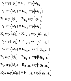
Fp = |Fp|exp(i) Structure factor of the protein
Fd = |Fd|exp(i) Structure factor of the isomor- phous derivative
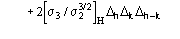
FH = Fd-Fp Structure factor of the heavy-atom structure (i.e. the atoms added to the native protein)

Ep = R exp(i) Normalized structure factor of the protein
Ed = S exp(i) Normalized structure factor of the isomorphous derivative
Np Number of non-H atoms in the primitive unit cell for the native protein
NH Number of heavy-atoms in the primitive unit cell for the derivative
 Zj = atomic number of the jth atom
 (Statistically equivalent) num-ber of atoms in the primitive unit cell
 Value of Neq for the native protein
 Value of Neq for the heavy atom structure
fj Atomic scattering factor of the jth atom
 The sum is extended to the native protein atoms
 The sum is extended to the heavy atom structure
 The sum is extended to the derivative atoms
 Ii = modified Bessel function of order i

 Derivative pseudonormalized structure factor

 Native pseudonormalized structure factor
 ,
,
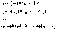
 Structure factor of a partial structure
 (Statistically equivalent) number of atoms of the partial structure for the
primitive unit cell.
(Statistically equivalent) number of atoms of the partial structure for the
primitive unit cell.
 (Statistically equivalent) number of atoms of the difference structure
obtained by subtracting the partial from the protein structure.
(Statistically equivalent) number of atoms of the difference structure
obtained by subtracting the partial from the protein structure.
 Structure factor of the protein structure pseudo-normalized with respect to
the difference structure.
Structure factor of the protein structure pseudo-normalized with respect to
the difference structure.
 Structure factor of the partial structure pseudo-normalized with respect to
the difference structure.
Structure factor of the partial structure pseudo-normalized with respect to
the difference structure.
APP Avian pancreatic polypeptide [11].
BPO Bacterial haloproxidase from Streptomyces aurefaciens [12].
E2 Catalitic domain of Azoto-bacter vinlandii dihydrolipoyl transacetylase [13].
M-FABP Recombinant human muscle fatty-acid-binding protein [14].
NOX NADH oxidase from Thermus thermophilus [15].
The relevant parameters characterizing the diffraction data of our test structures are given in Table 1.
of the phasing process. The problem was reconsidered by
Table 1 Relevant parameters for the diffraction data of our test structures. NREFL is the number of measured reflections up to the resolution RES for the native and derivative structures.
                           Native                             Derivative
Structure code      RES(Å)        NREFL        Heavy atom      2H/2p     RES(Å)       NREFL
APP                  0.99         17058            Hg          0.055      2.00        2086
BPO                  2.35         23956            Au          0.028      2.78        15741
E2                   2.65         10391            Hg          0.021      3.00        9179
M-FABP               2.14         7595             Hg          0.015      3.00        7125
NOX                  3.00         4295             Pt          0.041    3.00          4295
Giacovazzo, Cascarano & Zheng [18]: the distribution
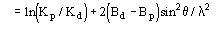
 (1)
(1)
was obtained for the case "native heavy-atom derivative", where
 (2)
(2)
and
 is the pseudo-normalized difference (with respect to the heavy-atom structure).
Since
is the pseudo-normalized difference (with respect to the heavy-atom structure).
Since
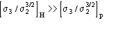 ,
the Cochran parameter is often negligible with respect to the term including
pseudonormalized differences: this last may attain large values even for large
proteins. Since
,
the Cochran parameter is often negligible with respect to the term including
pseudonormalized differences: this last may attain large values even for large
proteins. Since
 ,
may be positive or negative, positive as well as negative triplets can be
identified via (2).
,
may be positive or negative, positive as well as negative triplets can be
identified via (2).
Papers I-VI were devoted to describing a procedure for phasing, via distribution (1), all the reflections up to derivative resolution. The procedure succeeded with experimental data and may be described in a few steps.
 (3)
(3)
Actually from (3) the ratio Rk=Kd/Kp and the difference B=Bd-Bp are obtained. Then Bd and Kd are set to Bd=Bp+B and Kd=KpRk. Equation (3) is not sufficient for a correct rescaling of derivative data on protein data: some supplementary steps are needed. Since

one should expect that
 .
.
Therefore the values are rescaled by the factor
 (4)
(4)
to make the experimental distribution of
 closer to the expected one.
The application of (4) does not guarantee a good rescaling mostly when the derivative resolution is equal to or lower than 4 . A big improvement was obtained when the scaling was performed by exploiting the P() distribution (see papers III and V). From the joint probability distribution
one obtains
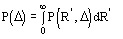 (5a)
(5a)
for positive values of and
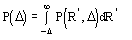 (5b)
(5b)
for negative value of (the limits of integration are because
 has
to be positive).
has
to be positive).
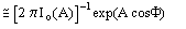
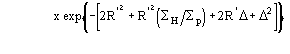
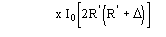
The distribution P() has been calculated (see paper III) by numerical methods:
we show in Fig.1 curves corresponding to various values of
 .
.
Let us now show how P() can be used in the normalizing process. Let T be a
positive threshold for ,
 be
the number of positive 's for which > T ,
be
the number of positive 's for which > T ,
 be the number of negative for which ||>T. Since P() is not an even
function, the ratio
be the number of negative for which ||>T. Since P() is not an even
function, the ratio
is expected to be larger than unity for any value of and for any T.

Figure 1 P() distribution for select values of
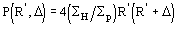
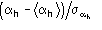
In Fig.2 we show RPM curves for different values of . RPM increases with and, for a given , increases with T. Its value is strictly correlated with the ratio kd /kp : errors in the estimate of this ratio will produce anomalous values of RPM. For example, if Fd values are scaled so that they are larger than their true values, the number of positive 's will exceed the expected value. In the converse case the number of negative 's will be larger than the expected value. In practice, the experimental P() curve is modeled by different sources of errors: besides the scaling error, also icorrect estimates of the difference Bd -Bp (as a consequence of the scaling error, errors in measurements, lack of isomorphism, etc.) will generate anomalies in P().
The above considerations suggest that histogram-matching techniques can be usefully applied to transform the experimental curve into the P() distribution expected at the chosen value. The resulting values will then be introduced into (1) for obtaining more accurate triplet invariant estimates.
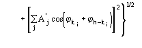
 ,
(6)
,
(6)
where j is defined by the equation [20]
and
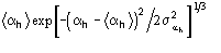
The reliability parameter h of any determined phase h is modified according to the agreement between the calculated and the expected value of h. In particular, if h is larger than the expected value
 ,
,
then the calculated h is replaced by
 ,
,
where
 .
.
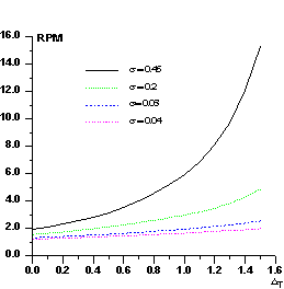
Figure 2 RPM curves for some representative values of against the threshold T.
The weighting scheme is designed to drive phases towards values that mimize the
difference between and
 by reducing in the tangent refinement the importance of the phases with too
large values of .
by reducing in the tangent refinement the importance of the phases with too
large values of .
In one possible strategy for the phase determination one could simultaneously apply the tangent formula (6) to all the reflections up to derivative resolution. Such a strategy would require the calculation of several tens of millions of triplets, their cumbersome management by the tangent formula and large storage and computing time.
We have chosen a different strategy: first we phase a small set of reflections
with large
 and R values ( i.e., batch 1, with NLAR reflections). The strategy is a
multisolution one: a starting set of phases are generated by a random process
[21]. Random phases are given to NLAR/2 reflections [22] with unit weights for
the origin and enantiomorph-fixing reflections, and with weights equal to 0.8
for the others. Cycles of weighted tangent refinement are first applied to the
NLAR/2 reflections and, after convergence, the phasing process is extended to
all the NLAR reflections.
and R values ( i.e., batch 1, with NLAR reflections). The strategy is a
multisolution one: a starting set of phases are generated by a random process
[21]. Random phases are given to NLAR/2 reflections [22] with unit weights for
the origin and enantiomorph-fixing reflections, and with weights equal to 0.8
for the others. Cycles of weighted tangent refinement are first applied to the
NLAR/2 reflections and, after convergence, the phasing process is extended to
all the NLAR reflections.
Among the various trials provided by the multisolution approach, the most probable one (on the basis of the figures of merit: see below) is used as a seed for phasing the remaining reflections. Batches of about 200 reflections, chosen in decreasing order of ||, are progressively phased via a phase extension procedure from batch number one.
The first FOM is
 ,
where
,
where

and
MABS gives a measure of the consistency of the triplet estimates, but it is not used as an active FOM for picking (in combination with others) the correct solution.
The second FOM (i.e., ALFCOMB) depends on the ratio
 ,
where
,
where
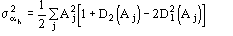
 is given in [[section]]3.2. This expression for the variance holds in the
absence of errors in measurements and in their mathematical treatment as well
as in the presence of perfect isomorphism between native and derivative
structures. If this is not the case, as with real data, the variance cannot be
perfectly calculated and is probably underestimated by
is given in [[section]]3.2. This expression for the variance holds in the
absence of errors in measurements and in their mathematical treatment as well
as in the presence of perfect isomorphism between native and derivative
structures. If this is not the case, as with real data, the variance cannot be
perfectly calculated and is probably underestimated by
 .
Accordingly, we used
.
Accordingly, we used
 instead of
 in ALFCOMB.
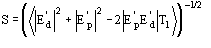
The third FOM (PSICOMB) relies on the expectation that the distribution of the
psi-zero triplets should be as random as possible. PSICOMB depends on the ratios
 ,
where
,
where

 .
.
The weak reflections that constitute psi-zero triplets with the NLAR
reflections are characterized by small values of both R and
 .
Here, there is no room for a FOM based on classical negative quartet estimates
based on native data only, which is unreliable for macromolecular structures of
usual size.
.
Here, there is no room for a FOM based on classical negative quartet estimates
based on native data only, which is unreliable for macromolecular structures of
usual size.
In our procedure negative and positive triplets play a similar role: they are
nearly equal in number and reliability, and are both actively used in the
phasing process. We decided to use the ratio
 as a FOM (CPHASE) involving both positive and negative estimated triplet phases
 .
.
A combined figure of merit (CFOM) integrates the indications arising from ALFCOMB, PSICOMB and CPHASE. The combination of the various FOMs involves suitable weights which indicate our confidence in them. CFOM allows a satisfactory discrimination of correct versus wrong solutions (see Table 2 for some results). For all the test structures the highest CFOM solutions are the correct ones: in the Table 2 they are marked by bold characters. We note: i) figures in Table 2 refer to batch 1, as explained in [[section]]3.2. ii) in the last column the average phase error (ERR) is shown. It is sufficiently small for all the test structures but NOX. iii) The solution is found in few trials. For all the test structures the maximum number of trials we explored was 100. We don't claim that correct solutions always correspond to the highest CFOM values. Severe lack of isomorphism, errors in measurements and/or in the treatment of the experimental data will reduce the efficiency of the procedure.
Table 2 FOM values for the `best' trial solutions as ranked by CFOM for the various test structures
APP
   Trial     MABS         ALFCOMB      PSICOMB      CPHASE       CFOM         ERR
    14          1.10      0.23         0.54         0.91         0.49         30
    28          1.10      0.23         0.53         0.91            0.49          30
     7          1.10      0.22         0.47         0.91            0.47          82
    29          1.09      0.20         0.46         0.91            0.46          83
    24          0.75      0.00         0.68         0.68         0.43         84
BPO
    18          0.84      0.40         0.96         0.75            0.63          29
     6          0.58      0.15         0.80         0.57            0.48          84
    19          0.58      0.14         0.79         0.57         0.48         83
E2
    24          1.14      0.75         1.0          0.89         0.76         27
     1          1.14      0.75         1.0          0.89            0.76          27
    22          1.14      0.75         1.0          0.89            0.76          27
     9          2.05      1.0          0.67         1.0             0.74          86
    16          2.05      1.0          0.66         1.0             0.73          86
    31          0.56      0.14         0.76         0.53         0.46         78
M-FABP
    24          0.85      0.10         0.57         0.77         0.44         39
    12          0.72      0.02         0.55         0.69         0.39         63
     6          0.64      0.01         0.54         0.64         0.38         83
NOX
    61          0.75      0.01         0.78         0.64            0.45          52
    65          0.75      0.01         0.78         0.64            0.44          52
    93          0.75      0.01         0.74         0.64            0.43          53
    66          0.65      0.00         0.74         0.58         0.42         63
The solution may then not be recognizable by the figures of merit, and may be characterized by a high value of ERR. In extremely unfavourable cases the correct solution could not be obttained at all.
When the solution is not clearly recognizable, a further check can be used:
a) Difference Fourier synthesis with coefficients
 are calculated for the solutions with the highest values of CFOM. The maxima of
the map should provide heavy-atom positions.
are calculated for the solutions with the highest values of CFOM. The maxima of
the map should provide heavy-atom positions.
b) Such parameters are refined according to the phase refinement process [25].
c) If the refined positional parameters coincide with an allowed origin of the protein space group, then the trial solution is discarded from the set of reliable ones.
Steps a), b) and c) are executed in sequence without user intervention.
Why should such a process work? Readers accustomed to direct phasing of small molecules know that in symmorphic space groups the so-called `uranium solution' occurs quite frequently. It is marked by a high consistency of triplets phases, which are all close to zero. An observed Fourier synthesis would produce a huge maximum at an allowed origin. This type of false solution may be recognized and therefore discarded by special FOMs like the psi-zero and negative-quartet criteria. Since the psi-zero FOM described in paper II is not highly discriminating for macromolecules and the negative-quartet criterion is not among the used FOMs, the calculation of the difference Fourier synthesis for proteins is an efficient substitute for the specific FOMs. It is worthwhile emphasizing that a difference Fourier synthesis should not provide huge maxima at the allowed origins as for small molecules: since our phasing procedure uses a nearly equivalent number of positive and negative triplets, peak intensities in the maps corresponding to the `uranium solutions' are similar to peak intensities corresponding to true heavy-atom positions.
In Table 3, we show, for each test structure and for trial solutions highly ranked by CFOM, but corresponding to true or "uranium" solutions, the heavy-atom positions as obtained after some cycles of Fourier-least-squares calculations. Trials 7 and 29 for APP, 9 and 16 for E2, show maxima at allowed origins and could therefore be discarded. This increases the discriminating power of CFOM. It may be concluded that in general, if use is made of the above considerations, the correct solution can be found with higher reliability among the different trials.
Table 3 Heavy-atom positions for each test structure and for trial solutions highly ranked by CFOM (compare with Table 2). The correct solutions are in bold characters.
  Structure    Trial   Heavy-atom position
    Name
APP            14 28    0.246 0.009 0.227
                7 29    0.244 0.010 0.226
                        0.000 0.390 0.500
                        0.000 .0396 0.500
BPO              18     0.591 0.026 0.279
                        0.221 0.112 0.311
E2              24 1    0.203 0.070 0.214
                22 9    0.203 0.069 0.213
                 16     0.203 0.070 0.215
                        0.000 0.000 0.500
                        0.000 0.000 0.500
M-FABP           24     0.609 0.441 0.742
NOX            61 65    0.393 0.242 0.524
                 93     0.393 0.242 0.524
                        0.893 0.242 0.225
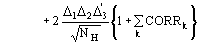
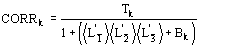
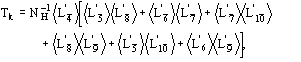
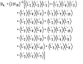
The highest CORR values are obtained for E2 and BPO, the derivatives of which are of extremely high quality. The worst phase values were obtained for NOX: the Pt derivative we used, as well as the other four derivatives of NOX, show serious lack of isomorphism [15].
Figure 3a BPO- section y=0 of the map obtained by Direct Methods.
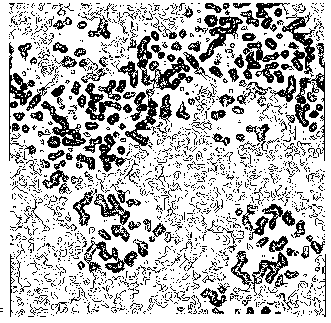
Figure 3b BPO- section y=0 of the true (obtained from the published model) map.
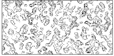
Figure 4a MFABP - section y=0 for the map obtained by Direct Methods.
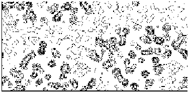
Figure 4b MFABP- section y=0 for the true (obtained from the published model) map.
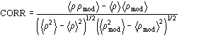
Table 4 Mean phase error (ERR) for the test structure up to derivative resolution. NREF is the number of phased reflections up to derivative resolution. CORR is the correlation factor between direct methods map (derivative resolution) and "true" map (native resolution).
Structure     NREF     ERR(Weighted)   CORR
   Name
APP           1850        61 (57)     0.3927
BPO           12774       57 (52)     0.4490
E2            6575        57 (52)     0.5121
M-FABP        5456        64 (61)     0.3733
NOX           4066        73 (69)     0.3129
Several techniques for improving direct-method phases by incorporating the heavy-atom structure have been proposed: particularly notable are those proposed by Fortier, Moore & Fraser [26] and by Klop, Krabbendam & Kroon [27]. None of these methods were useful at this stage: the above techniques seem to work well when careful phase estimates are available, and at this stage this is not the case. However in a paper in preparation (Giacovazzo & Siliqi) it is shown that heavy-atom substructure can in favourable cases lead to a notable improvement of the phases determined as in section 4.
We show in Table 5 the mean-phase errors and the CORR values obtained when the heavy-atom substructure is available (to be compared with Table 4).
In terms of CORR only APP and M-FABP show remarkable improvement of the electron density map. In the other cases, the information of the heavy atom structure does not produce any improvement in term of CORR index, but reduces the heavy-atom residual in the electron density map. Accordingly, the new phases proved to be a better starting point for the application of techniques devoted to extending phases up to native resolution: we refer mostly to solvent flattening [28], [29] and histogram matching techniques [30], [31].
Table 5 Mean phase error (ERR) when the information on the heavy-atom structure has been exploited (data up to derivative resolution). NREF is the number of phased reflections up to derivative resolution. CORR is the correlation factor between direct methods map (derivative resolution) and "true" map (native resolution)
Structure     NREF     ERR(Weighted)   CORR
   Name
APP           1854        58 (53)     0.4667
BPO           12613       57 (48)     0.4525
E2            6408        56 (47)     0.5026
M-FABP        5616        64 (59)     0.3992
NOX           4006        74 (67)     0.2939
In the same paper by Giacovazzo & Siliqi, an innovate solvent-flattening procedure has been settled, which carefully extends and refines phases up to the native resolution. For our test structures, we show in Table 6 the final correlation values between our final electron density maps and the "true" maps. All the maps but NOX are easily interpretable, as is suggested by the high values of CORR. The serious lack of isomorphism of the Pt derivative of NOX did not allow the method to produce batch one phases sufficiently good to be used as a seed for subsequent expansion. NOX will be a useful test when two or more derivatives will be used by our direct methods procedure.
Table 6 Mean phase error (ERR) after the application of our solvent-flattening procedure: phase has been extended to the set of data up to native resolution. NREF is the number of phased reflections up to native resolution. CORR is the correlation factor between our final map and the "true" map.
Structure     NREF     ERR(Weighted)   CORR
   Name
APP           17058       51 (44)     0.8150
BPO           23956       52 (46)     0.7391
E2            10391       41 (38)     0.8761
M-FABP        7589        53 (46)     0.7093
NOX           4619        77 (74)     0.2743
To allow the reader to check the quality of the new maps we show: a) in Figs. 5a and 5b the APP skeleton obtained
from our map and from the "true" map respectively; b) In Figs. 6, 7a and 8 some sections of our electron density maps for BPO, E2 and M-FABP (to be compared with true electron density map sections shown in Figs. 3b, 7b and 4b respectively).

Figure 5a APP skeleton from our map (visualized by RasMol v2.3 by Roger Sayle)
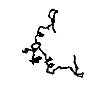
Figure 5b APP skeleton for the "true" map (visualized by RasMol v2.3 by Roger Sayle)
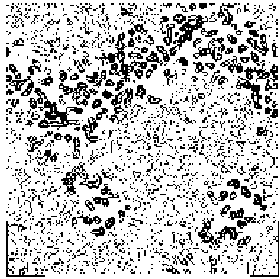
Figure 6 BPO section y=0 for the map obtained by applying our solvent flattening procedure to our Direct Methods map
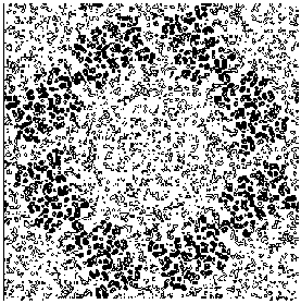
Figure 7a E2 section y=0.3 for the map obtained by applying our solvent flattening procedure to our Direct Methods map.
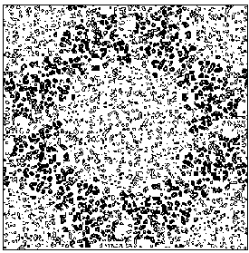
Figure 7b E2 section y=0.3 of the true (obtained from the published model) map.
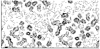
Figure 8 M-FABP section y=0 for the map obtained by applying our solvent flattening procedure to our Direct Methods map
 ,
become, as soon as this supplementary information is available, relations of
,
become, as soon as this supplementary information is available, relations of
order
 .
Since
.
Since
 the triplet reliability increases, and the protein structure becomes solvable
by direct methods. The above complexity reduction suggests that paraphernalia
used with great success to solve small molecules could be resuscitated for
application to macromolecules. A special wide-use and efficient tool is the
theory of representations by Giacovazzo [32], [33] (see also Hauptman [34] for
a related principle). The problem may be so stated: can we, for any phase
invariant , arrange the (R, S) space in a sequence of subsets, each contained
within the succeeding one and having the property that may be estimated, in
order of expected effectiveness, from the (R, S) magnitudes constituting the
subset? A solution to this question for SIR and OAS methods has been provided
by Giacovazzo [35]. For the quartet invariant
the triplet reliability increases, and the protein structure becomes solvable
by direct methods. The above complexity reduction suggests that paraphernalia
used with great success to solve small molecules could be resuscitated for
application to macromolecules. A special wide-use and efficient tool is the
theory of representations by Giacovazzo [32], [33] (see also Hauptman [34] for
a related principle). The problem may be so stated: can we, for any phase
invariant , arrange the (R, S) space in a sequence of subsets, each contained
within the succeeding one and having the property that may be estimated, in
order of expected effectiveness, from the (R, S) magnitudes constituting the
subset? A solution to this question for SIR and OAS methods has been provided
by Giacovazzo [35]. For the quartet invariant

the first subset of magnitudes to exploit for the SIR case is
 .
(7)
.
(7)
For the triplet invariant the second representation will involve the subset

 (8)
(8)
where k is a free vector.
Such a procedure exploits for (8) the special quintets
 ,
,
 ,
,
 ,
,
 ,
,
 ,
,
....................
etc., where the quintets are obtained by permutation of and .
The calculation of the joint probability distribution function
 (9)
(9)
for quartets, and the derivation of the distribution
 (10)
(10)
for triplets, are quite complicated. However a technique has been recently settled [36], [37], [38] which allows such calculations.
 ,
,
 ,
,
 ,
,
 ,
,
 ,
,
 ,
,
 ,
,
 ,
,
 ,
,
 ,
,
 ,
,
 ,
,
 ,
,
The conclusive conditional formula is
 (11)
(11)
where
(12)
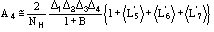
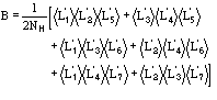
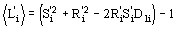
The main features of the formula may be so described:
a) the relation is of the order
 .
Since
.
Since
 is usually small, quartets are expected to be reliable (at least in
principle).
is usually small, quartets are expected to be reliable (at least in
principle).
b) the sign of A4 is determined by the product of two factors: the first is
 ,
which may be positive or negative, the second is the term
,
which may be positive or negative, the second is the term
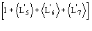 which again may be positive or negative.
c)
 is the expected value of
 In absence of prior information on the heavy-atom structure
 may only be estimated by probabilistic considerations [that is, by the formula
(12)]. Errors in measurements, lack of isomorphism, etc., can make
may only be estimated by probabilistic considerations [that is, by the formula
(12)]. Errors in measurements, lack of isomorphism, etc., can make
 remarkably different from
 .
In these cases quartet estimates are expected to be wrong. Once the heavy-atom
structure becomes available, A4 may be replaced by
.
In these cases quartet estimates are expected to be wrong. Once the heavy-atom
structure becomes available, A4 may be replaced by
 (13)
(13)
where
 Then quartet reliability proved to be comparable with triplet reliability. We
show in Table 7 for some test structures the statistical calculations for
assessing the reliability of the quartets having negative values of
Then quartet reliability proved to be comparable with triplet reliability. We
show in Table 7 for some test structures the statistical calculations for
assessing the reliability of the quartets having negative values of
Table 7 Statistical calculations for small-cross quartets by (13) (observed data).
             APP                            E2                          M-FABP
   NR          %        |4|0        NR         %        |4|0        NR      %            |4|0
  3621       71.6     114        10079        65.6       108     10084        54.9        96
  1577       75.7     119        2224         74.8       118     1993       57.7       95
   181       86.7     131        78           87.2       127     268        54.5       93
    5        80.0     142                                        47         63.8       89
                                                                 13         69.2       85
Table 8 BPO: statistical calculations for triplet invariants (found among the 1500 reflections with the largest of ||) relative to the formulas (2) and (15). Observed data for native and derivative structures are used.
   (2) Positive estimated         (15) Positive      (15) Negative
          triplets             estimated triplets    estimated triplets
 ARG      NR    %        ||0      NR    %        ||0      NR    %        ||0
 0.2    25195   68      69      20107   72      65      2785    52      92
 1.2     8680   72      64      10145   77      59      676     58      100
 3.2      0     -       -       531     84      50      30      40      98
 4.4      0     -       -       70      90      44      2       50       116
   (2) Negative estimated         (15) Positive      (15) Negative
          triplets             estimated triplets    estimated triplets
 ARG      NR    %        ||0      NR    %        ||0      NR    %        ||0
 0.2    24805   68      110     2739    51      89      19688   71      115
 1.2     6919   72      115     581     58      82      9485    76      120
 3.2      0     -       -         27      74    61      437     80      126
 4.4      0     -       -       8       75      67      45      78      122
Table 9 E2: statistical calculations for triplet invariants (found among the 855 reflections with the largest of ||) relative to the formulas (2) and (15). Observed data for native and derivative structures are used.
   (2) Positive estimated         (15) Positive      (15) Negative
          triplets             estimated triplets    estimated triplets
 ARG      NR    %        ||0      NR    %        ||0      NR      %      ||0
 0.2    25058   72      65      19537   79      57      2967    62      104
 1.2     4281   81      54      8088    85      50      599     74      119
 3.2      0       -     -       239     95      36      21      91      146
 4.4      0     -       -       30      100     23      1       100     159
   (2) Negative estimated         (15) Positive      (15) Negative
          triplets             estimated triplets    estimated triplets
 ARG      NR    %        ||0      NR    %        ||0      NR      %      ||0
 0.2    24942   71      114     2961    64      74      19234   78      122
 1.2     3234   81      126     531     75      62      7161    85      131
 3.2      0       -     -       27      85      56      207     94      143
 4.4      0     -       -       7       86      55      17      100     157
The conclusive formula estimating the triplet invariant may be written as
 (14)
(14)
where
 (15)
(15)
 We observe:
a) the distribution (14) is a von Mises-type function: it is unimodal, and the expected value of is 0 or according to whether A is positive or negative.
b) for proteins the term
 is quite often negligible with respect to the second term in (15). It can be
neglected.
is quite often negligible with respect to the second term in (15). It can be
neglected.
c) the contribution from the second phasing shell can change the value of the
expected phase. According to the first representation formula, is expected to
be zero if
 is positive, is expected to be if
 is negative. In the second representation formula the term
 may be considered a correction term which modulates the first representation
estimate. If
may be considered a correction term which modulates the first representation
estimate. If
 the
second representation estimate is different by from the first representation
estimate.
the
second representation estimate is different by from the first representation
estimate.
As in the quartet case
 is an estimate of
 ,
which may fail when lack of isomorphism and/or errors in the experimental data
occur. If the heavy-atom structure is available then
,
which may fail when lack of isomorphism and/or errors in the experimental data
occur. If the heavy-atom structure is available then
 may be used instead of
.
We show in Tables 8 and 9 the applications of (15) to E2 and BPO experimental
data. The data should be read as follows: triplet estimated positive by (2) are
split by (15) in positive and negative estimated triplets. Analogously,
triplets estimated negative by (2) are splitted by (15) in positive and
negative subsets. It is evident that (15) is more efficient than (2) in ranking
triplet reliability and in estimating their cosine sign. A useful practical
detail is that the results in Tables 8 and 9 are obtained by exploiting only
(about) 20 quintets per triplet.
may be used instead of
.
We show in Tables 8 and 9 the applications of (15) to E2 and BPO experimental
data. The data should be read as follows: triplet estimated positive by (2) are
split by (15) in positive and negative estimated triplets. Analogously,
triplets estimated negative by (2) are splitted by (15) in positive and
negative subsets. It is evident that (15) is more efficient than (2) in ranking
triplet reliability and in estimating their cosine sign. A useful practical
detail is that the results in Tables 8 and 9 are obtained by exploiting only
(about) 20 quintets per triplet.
 (16)
(16)
If the known partial structure is negligible (in terms of number of electrons) with respect to the complete structure then
and (16) reduces to Sayre's equation.
In terms of phases (16) is equivalent to
(17)
where
 is
the most probable value of
is
the most probable value of
 and
and
 (18)
(18)
is its reliability parameter.
Equation (16) has been recently reconsidered with respect to its possible use
in macromolecular crystallography. In a feasibility study by Giacovazzo &
Gonzalez-Platas [10], experimental tests on protein data show that the formula
is potentially able to estimate phases accurately, provided 30-40% of the
electron density is correctly located. Real cases were not examined. In the
future, eq. (16) will be applied to a situation frequently occurring in
practice: phase extension from derivative to native resolution, and phase
refinement. The use of (16) is the reciprocal counterpart of electron density
modification techniques. Indeed a basic step of these techniques is to fix
criteria to define the structure part, say
 ;
by Fourier inversion is calculated. Once this has been made is used, in
combination with the old values, as better approximation of the true phase
value.
;
by Fourier inversion is calculated. Once this has been made is used, in
combination with the old values, as better approximation of the true phase
value.
On the other hand (16) comes from the electron density squaring under the prior
condition that
 is known. The supplemental contribution of order
 comes from the squaring of the unknown part of the structure under the
restraint that
comes from the squaring of the unknown part of the structure under the
restraint that
 is known. To devise the optimal use of (9) for practical cases is not
straightforward, because it involves good approximations of the phases
is known. To devise the optimal use of (9) for practical cases is not
straightforward, because it involves good approximations of the phases
 and
and
 (which are not always available). Presently we are exploring different
approaches.
(which are not always available). Presently we are exploring different
approaches.
 (19)
(19)
where Q and
 can be defined in terms of the prior information, and the E's are the structure
factors normalized by taking the prior into account.
can be defined in terms of the prior information, and the E's are the structure
factors normalized by taking the prior into account.
In case a) the Main formula encompasses a previous Hauptman [41] formula [called B(z,t)] which is devoted to calculating the average of an exponential term which goes over all orientations of the triangle formed by three atoms:
 In case b),
 is expected to lie between 0 and 2: the use of such values and of the
corresponding reliability parameter should automatically translate the model
structure in the correct position.
is expected to lie between 0 and 2: the use of such values and of the
corresponding reliability parameter should automatically translate the model
structure in the correct position.
Additional phase relationships (which are not structure invariants or seminvariants) devoted to the translation problem were obtained by Giacovazzo [42] for polar space groups. In such cases the shift which brings a molecular fragment from a trial to the correct position may be restricted to a region which is smaller than the unit cell. For example, in P21 the origin may be freely chosen along the diad axis, and therefore may be restricted to the family of vectors [x 0 z]. This restriction is transformed, in the probabilistic approach, into supplemental prior information, so that one-phase, two-phase, three-phase relationships can be found (none of them being a structure invariant) which can be used for translating a molecule in the correct position. The Main formula (at least to the knowledge of the authors) has never been applied to proteins, or rotating nor for translating a molecule from a trial position. Giacovazzo's formulas were never applied to practical cases. In a forthcoming paper [43] it is shown that direct procedures can be successfully applied to macromolecules for translation purposes. We shortly quote here one of the experimental tests. M-FABP was originally solved by using multiple isomorphous replacement and molecular replacement procedures [14]. The model of adipocyte lipid binding protein (A-LBP), obtained from 2.5 resolution, was used as a search model from molecular replacement. The rotation function in MERLOT [44] was used to orient the molecule and a translation search was made by XPLOR [45] using 1351 reflections between 15 and 2.5 resolution. The same rotation procedure was followed in the paper by Giacovazzo, Manna & Siliqi, but the translation search was performed by direct methods. The solution with the highest CFOM corresponds to the correct translation. Our solvent-flattening procedure mentioned in section 5, automatically applied to direct-method phases, produced an electron density map having a correlation factor of 0.6 with the "true" map. In Fig. 9 we show the section at y=0.0 of the resulting electron density map, which may be usefully compared with the "true" section in Fig. 4b.
Figure 9 M-FABP section y=0 of the map obtained by translating via Direct Methods the model molecule, and subsequently, by applying our solvent-flattening procedure.
a) they are competitive with traditional isomorphous derivative techniques, with the supplemental appeal due to their high degree of automation;
b) they can profit from anomalous dispersion effects;
c) they can be applied to translating a molecule from a trial to the correct
position.
Only for point a), and particularly for the SIR case, has a well established
direct procedure been described. The MIR case however will easily follow. Point
b) is still at an earlier stage even if notable results have been obtained from
various authors. Point c) is starting. The rotation problem, so basic for the
molecular replacement area, has not been attempted for macromolecules by direct
methods. We intend to show that even in this area direct methods can offer an
important contribution.
The authors are grateful to Drs H.J. Hecht, W. Hol, A. Mattevi and G. Zanotti for having provided protein diffraction data and for useful discussions.
[2] Giacovazzo, C., Siliqi, D. & Ralph, A. (1994). Acta Cryst. A50, 503-510.
[3] Giacovazzo, C., Siliqi, D. & Spagna, R. (1994). Acta Cryst. A50, 609-621.
[4] Giacovazzo, C., Siliqi, D. & Zanotti, G. (1995). Acta Cryst. A51, 177-188.
[5] Giacovazzo, C., Siliqi, D. & Gonzalez-Platas, J. (1995). Acta Cryst. A51, 811-820.
[6] Giacovazzo, C., Siliqi, D., Gonzalez-Platas, J. Hecht, H., Zanotti, G. & York, B. (1995). Acta Cryst. D52, 813-825.
[7] Hauptman, H. (1982). Acta Cryst. A38, 632-641.
[8] Giacovazzo, C. (1983). Acta Cryst. A39, 585-592.
[9] Giacovazzo, C. (1983). Acta Cryst. A39, 685-692.
[10] Giacovazzo, C. & Gonzalez-Platas, J. (1995). Acta Cryst. A51, 398-404.
[11] Glover, I., Haneef, I., Pitts, J., Woods, S., Moss, D., Tickle, I. & Blundell, T. L. (1983). Biopolymers, 22, 293-304.
[12] Hecht, H., Sobek, H., Haag, T., Pfeifer, O. & Van Pee, K. H. (1994). Nature Struct. Biol. 1, 532-537.
[13] Mattevi, A., Obmolova, G., Schulze, E., Kalk, K. H., Westphal, A. H., De Kok, A. & Hol, W. G. J. (1992). Science, 255, 1544-1550.
[14] Zanotti, G., Scapin, G., Spadon, P., Veerkamp, J. H. & Sacchettini, J. C. (1992). J. Biol. Chem. 267, 18541-18550.
[15] Hecht, H., Erdmann, H., Park, H., Sprinzl, M., Schmid, R. D. & Schomburg, D. (1993). Acta Cryst. A49, Suppl. 86.
[16] Hauptman, H., Potter, S. & Weeks, C. M. (1982). Acta Cryst. A38, 294-300
[17] Fortier, S., Weeks, C. M., Hauptman, H. (1984). Acta Cryst. A40, 544-548
[18] Giacovazzo, C., Cascarano, G. & Zheng, C.-D. (1988). Acta Cryst. A44, 45-51.
[19] Blundell, T.L. & Johnson, L.N. (1976). Protein Crystallography, p. 336, London: Academic Press.
[20] Altomare, A., Cascarano, C., Giacovazzo, C., Guagliardi, A., Burla, M.C., Polidori, G. & Camalli, M. (1994). J. Appl. Cryst. 27, 435.
[21] Baggio, R., Woolfson, M.M., Declercq, J-P. & Germain, G. (1978). Acta Cryst. A34, 883-892
[22] Burla, M.C., Cascarano, G. & Giacovazzo, C. (1992). Acta Cryst. A48, 906-912.
[23] Cascarano, G., Giacovazzo, C. & Viterbo, D. (1987). Acta Cryst. A4843, 22-29.
[24] Cascarano, G., Giacovazzo, C. & Guagliardi, A. (1992b). Acta Cryst. A48, 859-865.
[25] Dickerson, R.E., Kendrew, J.C & Strandberg, B.E. (1961). Acta Cryst. 14, 1188-1195.
[26] Fortier, S., Moore, N. J. & Fraser, M. E. (1985). Acta Cryst. A41, 571-577.
[27] Klop, E. A., Krabbendam, H. & Kroon, J. (1987). Acta Cryst. A43, 810-820.
[28] Wang, B.C. (1985). In "Methods in Enzymology", Vol.115 (Wyckoff, H.W., Hirs, C.H.W. and Timasheff, S.N., ed.), p.90-112.
[29] Leslie, A.G.W (1987). Acta Cryst. A43, 41-46
[30] Lunin, V. Y (1993). Acta Cryst. D49, 90-99.
[31] Zhang, K.Y.J. & Main, P. (1990). Acta Cryst. A46, 41-46
[32] Giacovazzo, C. (1977) Acta Cryst. A33, 934-944
[33] Giacovazzo, C. (1980) Acta Cryst. A36, 362-373
[34] Hauptman, H. (1976). Acta Cryst. A32, 934-940
[35] Giacovazzo, C. (1984) International School of Crystallography, lecture notes, in Direct Methods of Solving Crystal Structures, Erice, Italy
[36] Giacovazzo, C. & Siliqi, D. (1996). Acta Cryst. A52, 133-142
[37] Giacovazzo, C. & Siliqi, D. (1996). Acta Cryst. A52, 143-151
[38] Giacovazzo, C. & Siliqi, D. (1996). Acta Cryst. A53, 000-000 (submitted)
[39] Kiriakidis, C.E., Peschar, R. & Shenk, H. (1996) Acta Cryst. A52, 77-87
[40] Main, P. (1976) Crystallographic Computing Techniques, edited by F. Ahmed, p 99-105, Copenhagen; Munskgaard
[41] Hauptman, H. (1965). Z. Krist. 121, 1-8
[42] Giacovazzo, C. (1988). Acta Cryst. A44, 294-300.
[43] Giacovazzo, C., Manna, L. & Siliqi, D. (1997) in preparation
[44] Fitzgerald, P.M.D. (1988). J. Appl. Cryst. 21, 273-278.
[45] Brnger, A.T. (1990) XPLOR version 2.1, manual. A system for crystallography and NMR.